Warning: include(): http:// wrapper is disabled in the server configuration by allow_url_include=0 in /home/www/blog.pecuniology.com/wp-content/themes/suffusion/header.php on line 71

Warning: include(http://www.pecuniology.com/inc/bannerButtons.php): failed to open stream: no suitable wrapper could be found in /home/www/blog.pecuniology.com/wp-content/themes/suffusion/header.php on line 71

Warning: include(): Failed opening 'http://www.pecuniology.com/inc/bannerButtons.php' for inclusion (include_path='.:/usr/local/php5.6/lib/php') in /home/www/blog.pecuniology.com/wp-content/themes/suffusion/header.php on line 71
Mar 152013
 

A personal finance question that is asked on many accounting and financial professional exams is the Lifetime Savings Problem, in which one is asked how much one would have to set aside on a regular basis, beginning in one’s youth, in order to enjoy a retirement of a particular level. A typical example is:

Imagine that you planned to retire 30 years from now, and that you wanted to set up an account, into which you would make equal-sized payments each year during your working years, that would enable you buy an annuity that would pay you $25,000 at the end of each year for the 25 years immediately after you retired. Based on the expectation that your savings account should earn 9% per annum and that the retirement annuity should have a more conservative yield to maturity of 3% per annum, how much should you set aside each year until your planned retirement?”

This problem is in two parts: a) your retirement plan, and b) your savings plan to achieve that goal.

Savings Plan

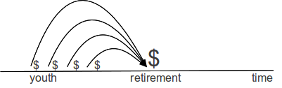
Pay into Retirement Account

Retirement Plan

Draw from Retirement Account

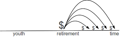
A financial arrangement like the ones depicted above, in which payments—called coupon payments (c) for historical reasons—are made on a regular schedule for a specified period of time (t) is known as an annuity*. Here, the retirement account is an annuity that will pay you (perhaps, you will buy it from an insurance company or a large bank), and the savings account is an annuity that you will pay into (perhaps, a brokerage account or a statutory retirement account that you manage with the help of a financial professional).

To solve this puzzle you need to work backwards, first by deciding how much you would like to receive each year after you retire and for how many years; then by calculating the expected value—the price that you expect to pay, when the time comes—of an annuity that will provide for your retirement, which value becomes your savings goal; and finally by calculating how much money you should set aside each year between now and retirement, in order to achieve that goal.

Before you can know how much (c) to pay each year into a savings account that you open in your early years, you need to know how much you want to save. In other words, the price (APV for “annuity present value”) of the annuity that you plan to buy when you retire—the price that you expect to have to pay upon retirement—is exactly equal to the amount that you need save (AFV for “annuity future value”) during your working years. Tomorrow’s present value (i.e., price) is today’s future value.

Retirement Plan

If you imagined, for planning purposes, that you could live on $25,000 (c) per year after you retire, and that you wanted to plan for a 25-year (t) retirement—on the expectation that you’ll figure out a Plan B sometime during the next 55 years, in case you live beyond Year 26 after retirement—and that you expected your retirement account to earn 3% (r) per year, then you would need to save (APV):

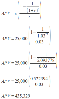
This means that you need to have $435,329 on the day of your retirement, 30 years from now, so that you can buy the annuity that will pay $25,000 per year for 25 years.

Savings Plan

In order to save that amount (AFV), you plan to make equal annual payments (c) for the next 30 years (t), and you expect that you can earn an average of 9% per year (r) over that time.

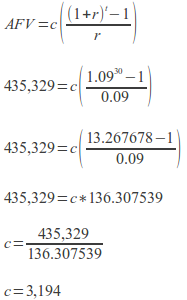
If all goes according to plan, then, if you set aside $3,194 at the end of every year for the next 30 years and earn an average of 9% per year on your savings, then you should have $435,329 in three decades that you can use to buy an annuity that pays $25,000 per year for 25 years.

Invest accordingly.

Prof. Evans


note: For a detailed explanation of annuities, review my “Time Value of Money” video lecture. If you have difficulty viewing the videos try using VLC Media Player, “a free and open source cross-platform multimedia player and framework that plays most multimedia files as well as DVD, Audio CD, VCD, and various streaming protocols.” [return to main text]

Dec 192012
 

17 December 2012, the San Francisco Chronicle had a story—”Solar Power Adds to Non-Users’ Costs“—that provides background for a very good Microeconomics test question:

Q: Under what circumstances can the combination of a decrease in demand and an increase in supply lead to an increase in prices?

The short answer, of course, is, “When government interferes with the market process.”

If you are required to show your work, here’s what you do:

First, note that the own-price demand elasticity for electricity tends to be low for most consumers, meaning that one tends to consume the same quantity, seemingly regardless of the price. For example, one would not expect someone to throw open the windows in the middle of summer, with the air conditioner turned to its lowest setting, if the price of electricity fell substantially. More likely one would continue to consume electricity at approximately the same rate and use the cost savings on something that had a higher own-price elasticity of demand, like those things that collect in one’s shopping cart at Amazon.com, but one rarely gets around to ordering for delivery.

You can illustrate it this way:

Vertical Demand Curve in Equilibrium

Fig. 1 : Vertical Demand Curve in Equilibrium

This is very similar to the textbook Supply & Demand graph, but with the Demand curve at the same quantity demanded for every price. (Of course, this is not realistic for all prices, and the real world is not so well-behaved. Such is the nature of economic models.)

As indicated in the article above, the increase in solar panels being installed on the roofs of residential and commercial buildings in California is causing a decrease in overall demand for conventional electricity.

In an unregulated market, we might illustrate it this way:

Vertical Demand Curve with Shift in Demand

Fig. 2 : Vertical Demand Curve with Shift in Demand

As the demand decreases, due to the existence of solar-powered substitutes, price tends to fall.  In an unregulated market, executives and shareholders in waning industries receive signals in the form of accumulating inventories—unsold output—that they either should reduce their prices, reduce their output, or both.  If the trend continues—as happened with sailing ships, tools for making whale oil, steam locomotives, buggy whips, etc. in earlier generations—the executives and shareholders receive signals that they should consider whether liquidating and reallocating their existing resources might be more profitable than clinging to a dying firm or industry.  (Schumpeter referred to this as ‘creative destruction‘.)

However, in a regulated market, suppliers and regulators agree on a price and fix it ex ante.  Typically, the price is below the equilibrium, at least in the first iteration, so that consumers will be happy and express their gratitude to the politicians who oversee the regulators.  (This sometimes is referred to as ‘the iron triangle‘ of regulation, and it is related to the concept of ‘regulatory capture‘.)

We can illustrate it this way:

Vertical Demand Curve with Regulated Price

Fig. 3 : Vertical Demand Curve with Regulated Price

Here, the regulated price (Pr) is below the equilibrium price that would clear the market, but is at least as high as is needed to generate sufficient revenues to cover the costs of production.  The executives and shareholders of regulated firms generally are rewarded for their cooperation with monopoly rights in the form of franchises that grant them the exclusive right to serve a particular geographic region.

The firm’s total revenue is illustrated as area of the pink rectangle below, which is price * quantity.  It is possible that a firm’s executives and shareholders might want to increase output, so that the firm could sell the excess into neighboring markets, but the jurisdictions of most regulated industries do not adjoin jurisdictions where competitors are unregulated.  Most likely, every neighboring territory is served by a different monopolist franchisee.

Vertical Demand Curve with Regulated Price / Total Revenue

Fig. 4 : Vertical Demand Curve with Regulated Price / Total Revenue

Returning to Fig. 2, as solar panels reduce demand for conventional electricity, the demand curve shifts to the left.

Vertical Demand Curve with Regulated Price and Demand Shift

Fig. 5 : Vertical Demand Curve with Regulated Price and Demand Shift

Because the electricity providers’ prices are fixed by regulation, and they have very high fixed costs, they are loath to lower their prices.  In fact, the fixed costs of maintaining a capital base that consists of indivisible centralized facilities, power lines, poles and waterproof underground conduits, substations, and other large and expensive infrastructure can vastly exceed the variable costs of fuel and peak-time labor, and these large fixed costs are the primary drivers of the price that suppliers and regulators agreed to previously.

Now, with a smaller consumer base, the utility operators have fewer customers to divide their fixed costs among.  In order to arrive at a rectangle with the same area as the pink one in Fig. 4, given that the utility operators not only cannot force consumers to buy conventional electricity, but are required to buy the excess electricity produced by the owners of the solar panels.  In other words, the suppliers are doubly pinched, and their only savings are in the form of electricity purchased at full retail from their customers, accompanied by a relatively slight decrease in variable fuel costs.

The only viable alternative in this situation is for the operators of the regulated conventional electricity utilities to petition the regulators for a price increase to be passed along to the remaining conventional electricity consumers.

Vertical Demand Curve with Regulated Price / Price Increase

Fig. 6 : Vertical Demand Curve with Regulated Price / Price Increase

Considering that solar energy becomes more economically viable, when its primary competitor—conventional electricity—becomes more expensive, the rising prices in this scenario create an incentive for even more consumers to adopt solar energy, thereby shifting the demand curve even further leftward toward zero… creating yet more upward price pressure.

And, in this way, regulation creates an environment, in which a decrease in demand can lead to an increase in price.

Invest accordingly.

Prof. Evans

Nov 262012
 

The vast majority of firms do not pay dividends, which renders the use of dividend discounting methods for estimating their values moot. In this case, one can use discounted expected cash flows: net income (NI), operating cash flows (OCF), or free cash flows (FCF), depending on the level of sophistication required by the analyst.  However, all of these require the analysis of the firm’s financial statements, which might involve more effort than one is willing to expend in a preliminary analysis.

With publicly traded firms that do not pay dividends, another option exists using the price/earnings ratio (P/E).

Remember that:

NI = Dividends + Retained Earnings

P/E = Equity/NI

NI is the pool of funds from which a firm would pay dividends if it paid dividends, and dividend discounting models assume that all of the value of the firm is paid out to shareholders in the form of a dividend (D).

In this way, we can see P/E = Equity/NI as being similar to P/E = price-of-equity (P) / D:

P/E = Price / Dividend = P / D

To use this in our dividend discount formula, we need to take the reciprocal:

P/E ratio discounting formula

where

re : return on equity / cost of equity
D : dividend
P : price
P/E : price/earnings ratio
g : growth rate

Start with the P/E ratio, take its reciprocal (1 ÷ P/E), multiply by (1+g), and then add g.

You can practice this in the WACC Quiz, by clicking the Practice link above.

I hope that this helps.

Prof. Evans